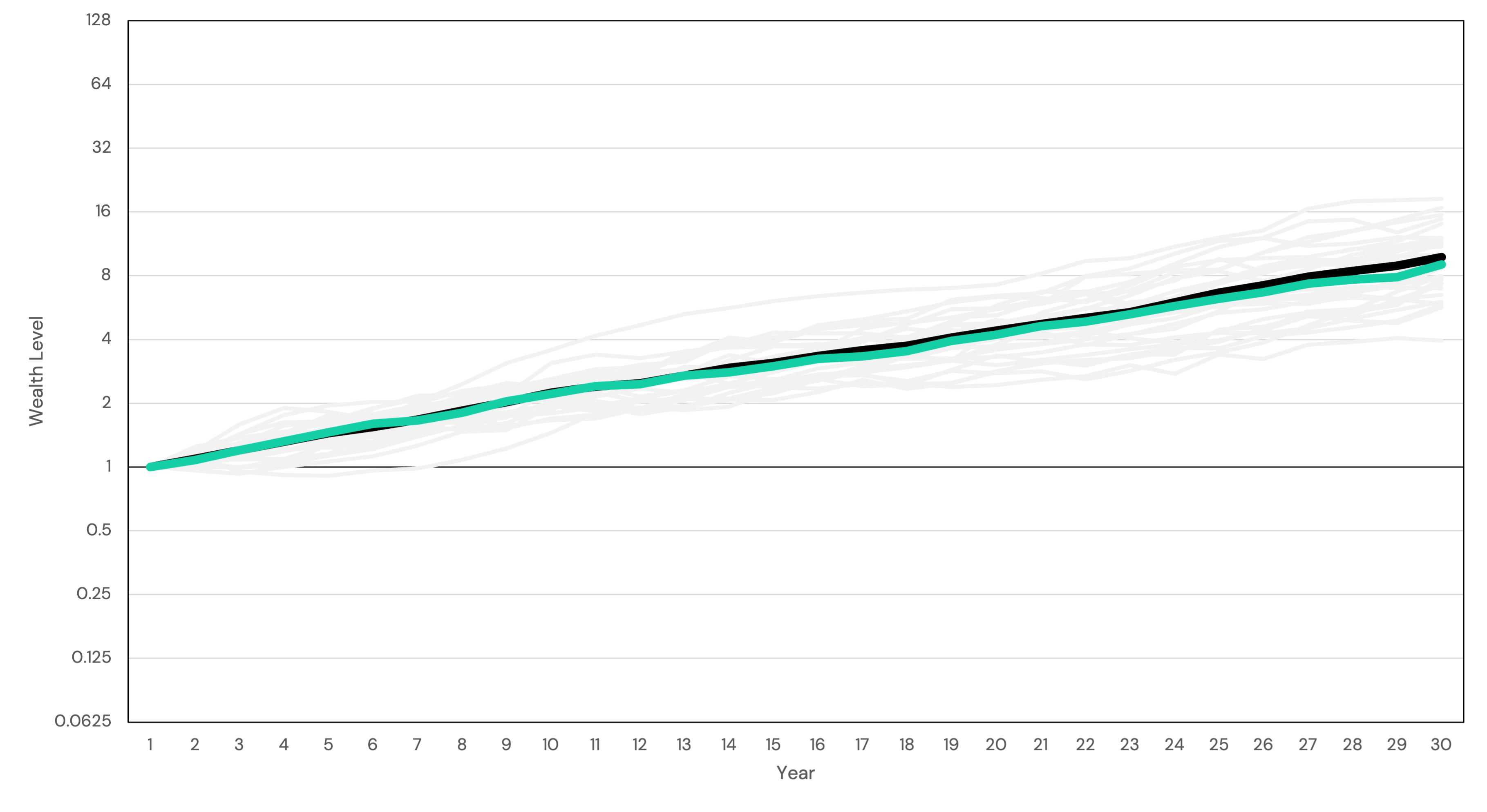
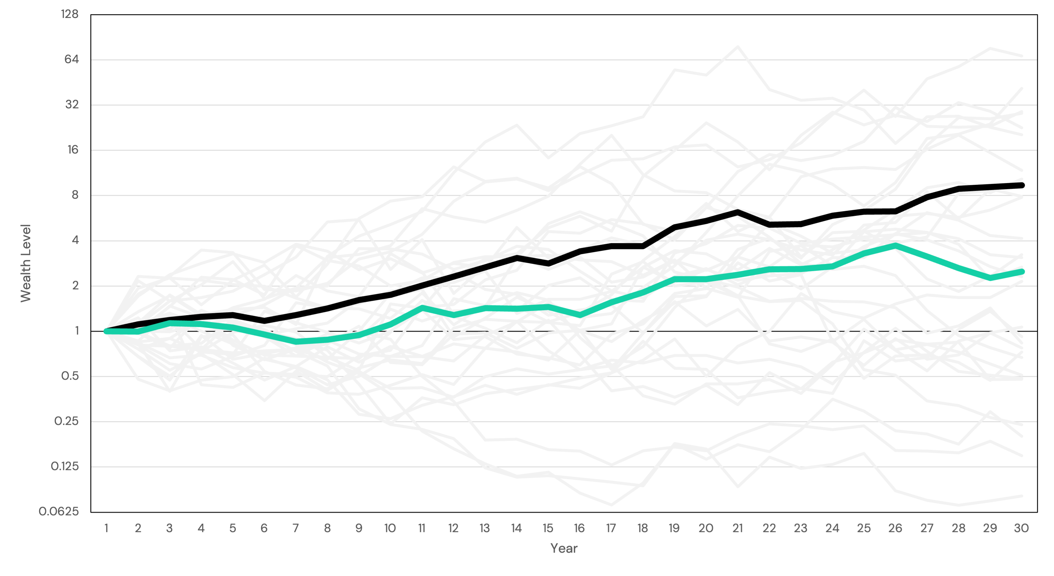
In financial planning, it is common to perform monte-carlo simulations, where potential wealth paths are projected into the future. Evaluating the average wealth path, however, may be highly misleading for setting expectations. In fact, if we only evaluate the average path, we find a somewhat counter-intuitive result: volatility doesn’t matter at all. However, because investors can only try to average their outcomes over time, and because wealth is a compounding process, it is not the average result that wealth converges towards, but rather the median. Volatility is a drag on the median outcome, aligning with our intuition that excessive volatility is dangerous to our long-term wealth.
Compound Growth, Volatility
The Misleading Mean
In the world of bell-curves and normal distributions, we typically expect experiences to be clustered around the average. For example, there are more people close to the average height than there are far away. In many cases, however, the so-called “average” can be entirely misleading for the experience you can expect.
Wealth distribution is a perfect example of this. According to the World Inequality Database, in 2021 in the United States, the top 1% of families held 35.3% of the wealth while the bottom 50% held 0.3%. If we take the aggregate net worth and divide by the number of adults, we arrive at an average around $500,000 per person. Adults in the bottom 50%, however, had a net worth closer to $14,500.
In other words, if you pick a random person off the street, their experience is likely much closer to $14,500 than $500,000. It’s the wealthy outliers that are pulling the average up. Way up. A more applicable metric, in this case, might be the median, which will say, “50% of experiences are below this level and 50% are above.”
And this makes some intuitive sense. Wealth has (for the most part) a lower bound at $0 but no real upper bound. The asymmetry allows the average to be very different than the median experience.
But when it comes to our own financial planning, which do we care about?
You Are Not a Monte-Carlo Simulation
The problem with running a simulation and talking about the average result is that we do not get to live the average path; we live a single path.
Under this context, risk aversion is not so foolish. If we have our arm mauled off by a lion on the African veldt, we cannot simply “average” our experience across the infinite universes of other potential outcomes where we may still have our limb. Rather, our state is permanently altered for life.
Similarly, if we lose 50% of our money on a bad investment, we cannot simply average our results across the multiverse of alternative selves who may not have lost theirs. The best we can do is try to average our results over time on our one, singular path.
When you average over time, choices compound. And when choices compound, so does risk.

Compounding at the Median
The impact of compounding means that volatility matters. Many investors may already be familiar with this idea under the name volatility drag or variance drain. The idea can be illustrated with a simple example. Consider the case where an investment goes up 100% on the first day and down 50% on the second day. The average return over the two days is 25%, but the compound return is 0%.
For less extreme examples, a larger number of periods is required for the effect to materialize. Regardless, the effect remains the same: volatility drives a wedge between average and compound. Consider these simple two-period examples:
| Year 1 | Year 2 | Average | Compound Rate |
| +10% | +10% | +10% | +10.0% |
| +15% | +5% | +10% | +9.9% |
| +30% | -10% | +10% | +8.2% |
| +50% | -30% | +10% | +2.5% |
In all four cases, the average return is 10%. However, as the volatility of the returns increases, the compound growth rate declines. Volatility pushes the compound rate further and further from the average.
Why do we care? Wealth is a compounding process, which means we do not expect our wealth to converge upon the average result over time, but rather the median result.
Tools Center:
Easily backtest & explore different return stacking concepts
Model Portfolios:
Easily backtest & explore different return stacking concepts
Future Thinking:
Receive up-to-date insights into the world of return stacking theory and practice
The Math Behind Wealth’s Growth Rate
In this section, we will prove that the wealth process converges on the median result over time. However, the math is not necessary for understanding the intuition and this section can be skipped for those less interested in the details.
As is common in finance, we will begin by assuming that wealth follows a geometric brownian motion. This means we can write our wealth process as:
As the wealth process follows a log-normal distribution, we know the median is:
The mean, however, is slightly different. Note that we can re-write the above wealth equation as:
Taking the expectation, we get:
Note that is just the expectation of a log-normal distribution with zero mean and a volatility of
. Thus, we find:
The important takeaway here is that volatility does not affect our expected level of wealth. It does, however, drive the mean and median further apart.
The intuition here is that while returns are generally assumed to be symmetric, wealth is highly skewed: we can only lose 100% of our money but can theoretically make an infinite amount. Therefore, the mean is pushed upwards by the return shocks.
Over the long run, however, the annualized compound return does not approach the mean: rather, it approaches the median. Consider that the annualized compounded return can be written:
Where is an i.i.d. standard normal and reflects the random shock on day
. As
goes to infinity, the second term approaches 1, leaving only:
Which is the annualized median compound return. Hence, over the long run, over a single realized return path, the investor’s growth rate should approach the median, not the mean. Volatility places a crucial role in long-term wealth levels.
(For a more thorough derivation, please see these excellent notes by Guillaume Rabault.)
Conclusion
In this post we strived to provide the intuition – and math – as to why volatility is a critically important ingredient in determining the long-run growth rate of an investor’s portfolio. By only looking at the average outcome of wealth simulations, investors may be misled into believing a much higher rate of return is achievable. However, because investors do not have the ability to average their results across a multiverse of different outcomes, but rather can only average their returns over time, risk has the opportunity to compound.
Counter to the expectation that higher risk should be compensated with higher reward, a reduction of volatility, even at the expense of a lower expected return, can lead to a higher level of wealth accumulation.
This can be non-intuitive. After all, how can a lower expected return lead to a higher level of wealth? Since wealth is a convex function of return, a single bad, outlier return can be disastrous. A 100% gain is great, but a 100% loss puts you out of business. While taking some risk is necessary to earn reward, excessive risk can lead to the permanent impairment of capital.


