Return Stacking and Volatility Drag

2023-07-13 | Education

Overview

A common critique against levered ETFs is that they are subject to volatility drag (sometimes referred to as variance drain). In this article, we briefly describe what volatility drag is, how it is magnified when leverage is applied, but how diversification can play an important role in reducing its impact.

Key Topics

Compounding, Volatility

What is Volatility Drag?

[latexpage]
Volatility drag – sometimes also referred to as “variance drain” – is the return difference that emerges between the average return of an asset or portfolio versus its compound growth rate.

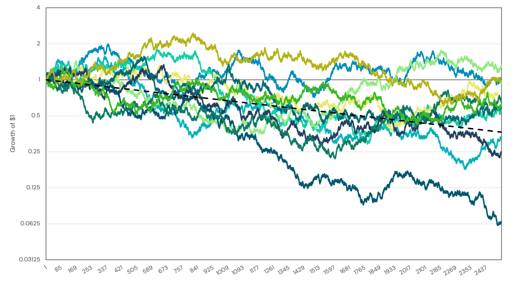
As an example, consider this very simple scenario: a stock that returns either +2% or -2%, with equal probability, every day. While the average daily return is 0%, the daily compound growth rate is -0.04% ( $\left((1+2\%)(1-2\%) \right)^{1/2} - 1$ ).

Despite having an average daily return of zero, over a long enough period, this hypothetical stock would go to zero.

Figure 1: Hypothetical, simulated returns of a stock that returns either +2% or -2%, with equal probability, every day. –Dashed line– plots -0.04% compound daily growth rate.

stock-simulations-and-volatility-drag-1024x560

Volatility drag emerges from the compounding process of returns. In his paper Variance Drain, Thomas Messmore derives that:

$r_{g} \approx r_{a} - \frac{\sigma^{2}}{2}$

Where $r_{g}$ is the compound growth rate, $r_{a}$ is the average return, and $\sigma$ is the volatility of the asset. The $- \frac{\sigma^{2}}{2}$ is the volatility drag (or variance drain) and it is easy to see that as $\sigma$ goes up, this drag gets bigger.

Register for our Advisor Center

Tools Center:
Easily backtest & explore different return stacking concepts

Model Portfolios:
Return stacked allocations, commentary and guidance designed
for a range of client risk profiles and goals

Future Thinking:
Receive up-to-date insights into the world of return stacking theory and practice

Volatility Drag in Levered ETFs

So what happens if we introduce leverage? We scale both the average return and the volatility. For a given leverage level $L$ , we are left with:

$r_{g} \approx L r_{a} - L^{2} \frac{\sigma^{2}}{2}$

Notice that the leverage term is squared in the volatility drag component. That means with a little bit of leverage, that term starts to grow very quickly.

$L = 1: r_{g} \approx r_{a} - \frac{\sigma^{2}}{2}$

$L = 2: r_{g} \approx 2 r_{a} - 4 \frac{\sigma^{2}}{2}$

$L = 3: r_{g} \approx 3 r_{a} - 9 \frac{\sigma^{2}}{2}$

$L = 4: r_{g} \approx 4 r_{a} - 16 \frac{\sigma^{2}}{2}$

We can see that our average return is scaled linearly but our volatility drag grows non-linearly. This does not mean leverage is inherently bad, though. For different combinations of $r_{a}$ and $ \sigma $ it is entirely possible that there are levels of leverage where the increase in expected returns more than offsets the added variance drag.

Leverage with Diversifying Assets

In the section above, we assumed we were using leverage to add more of the same thing. The math changes, though, if we are using leverage to introduce a new thing. For a portfolio of two assets, we have the basic portfolio math:

$r_{g} \approx (w_{1} r_{1, a} + w_{2} r_{2, a}) - \frac{(w_{1}\sigma_{1})^{2} + (w_{2}\sigma_{2})^{2} + 2 \rho w_{1} \sigma_{1} w_{2} \sigma_{2}}{2}$

Where:

$w_{1}$ and $w_{2}$ are the weights of the assets;
$r_{1,a}$ and $r_{2,a}$ are the expected returns of the assets;
$\sigma_{1}$ and $\sigma_{2}$ are their volatilities;
and $\rho$ is their correlation.

The biggest difference is in the volatility drag component. Assume, for a moment, that $w_{1} = w_{2} = 1$ , $r_{a} = r_{1,a} = r_{2,a}$ , and $\sigma = \sigma_{1} = \sigma_{2}$ . In other words, we’re adding 100% of the first asset and 100% of the second asset, and they have identical expected returns and volatilities.

If $\rho = 1$ , the whole equation simply collapses to the case above where $L = 2$ . Which makes sense, because the assets are basically the same.

But let’s say the correlation between the assets, $ \rho $, is equal to zero. We end up with:

$r_{g} \approx 2 r_{a} - \sigma^{2}$

Compared to the case where the correlation was 1, the volatility drag gets cut in half! In a more extreme case, we can consider what happens if correlation is -1.

$r_{g} \approx 2 r_{a}$

The volatility drag disappears entirely.

Conclusion

Volatility drag – or variance drain – applies to the return of all assets, whether they are levered or not. After all, it’s just the math of compounding returns.

When an asset’s returns are levered, however, volatility drag can play an increasingly important role in influencing returns.

This means that volatility drag absolutely applies to return stacked® ideas. However, if we are thoughtful not only about what we are stacking together, volatility drag can grow at a much, much slower rate than typical levered ETFs.

The simple takeaway is this: more volatility means more volatility drag. If you double your exposure through leverage, you quadruple your volatility drag. If you are able to layer on a negatively correlated asset, however, your portfolio volatility will go down, and with it your volatility drag.