Capital Market Assumptions when Return Stacking
Overview
Capital market assumptions (“CMAs”) are an important input in portfolio construction and financial planning. Given an existing set of CMAs, this article demonstrates how CMAs can be computed for return stacked® strategies.
Key Topics
Expected Returns, Variance, Correlations
Introduction
Many financial plans are built off the backbone of capital market assumptions (“CMAs”). These forecasts of asset class expected returns, volatilities, and correlations are critical inputs to the portfolio construction process. Without them it can be difficult to introduce a new exposure without ad hoc decisions, often formed on heuristics rather than informed analytics.
Fortunately, given a set of existing capital market assumptions, inferring the capital market assumptions of a return stacked® strategy is simple.
For the rest of the article, we will assume a generic return stacked® portfolio, P, that is 100% Asset A + 100% Asset B.
An Excel workbook implementing the math below is available for download here.
The Expected Return
The expected return of our portfolio is easy to calculate: it is the expected return of Asset A plus the expected return of Asset B minus our expected cost of financing/leverage and net of any fees.
We know from previous articles that the cost of leverage can often be approximated with the return of cash (i.e. short-term U.S. Treasury Bills). If we think it is appropriate, we can even add a constant premium to this cost (for example, when using S&P 500 futures as our source of leverage, the historic cost of leverage has been closer to U.S. Treasury Bills + 0.4%).
As an example, assume we have the following expected returns:
- Stocks: 7%
- Bonds: 5%
- Cash: 3%
Then the expected return of a return stacked® portfolio that is 100% Stocks + 100% Bonds would be:
7% + 5% – (3% + L) – C
Where L is any assumed cost-of-leverage premium and C is the cost of the product wrapper (e.g. the ETF expense ratio).
Register for our Advisor Center
Tools Center:
Easily backtest & explore different return stacking concepts
Model Portfolios:
Return stacked allocations, commentary and guidance designed
for a range of client risk profiles and goals
Future Thinking:
Receive up-to-date insights into the world of return stacking theory and practice
Volatility
Arriving at the expected volatility of our portfolio is slightly more complicated, but there is still a straightforward calculation.
We can calculate the variance of a two-asset portfolio as:

Where w is weight, σ is volatility, and ⍴ is correlation. We can trivially extend this to a three-asset portfolio as well:

Why would we need a three-asset portfolio? A three-asset portfolio allows us to explicitly model the cost-of-financing as an asset; i.e. we can think of our portfolio as 100% A + 100% B – 100% Financing. For volatility estimation purposes, we might consider using Cash as our proxy for Financing.
As an example, assume the following volatilities:
- Stocks: 15%
- Bonds: 6%
- Cash: 1%
We’ll also assume the following correlations:
- Stocks/Bonds: -0.3
- Stocks/Cash: -0.05
- Bonds/Cash: 0.1
Plugging all these values (A = Stocks, B = Bonds, C = Cash) into the equation above provides us with the variance of our portfolio. Taking the square root of this result provides our estimate for portfolio volatility. In this case, we estimate the portfolio volatility to be 14.4%.
The Return Stacking landscape is ever evolving, go deeper by connecting with a team member.
Cross-Asset Correlations
While correlations are the most complex result to arrive at, they can still be calculated with a single equation. (If you’re allergic to math, we’d recommend simply skipping to the example below.)
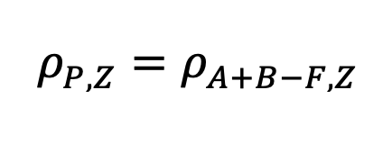
The correlation between our portfolio, P (100% A + 100% B – 100% Financing), and some asset, Z, is equal to:

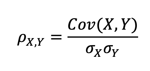
Recall that:

Where Cov(X,Y) is the covariance function. We can re-write our equation as:

We can re-write this further as:

Simplifying terms, we are left with:

All the terms in this equation should be given in our capital market assumptions (or calculable given the sections above), leaving us with our solution.
As an example, we will again assume a return stacked® portfolio that is 100% Stocks + 100% Bonds – 100% Financing where Financing can be proxied with Cash. Using the assumptions above, we can calculate the correlation to Bonds as:

Conclusion
In this article, we have outlined the equations necessary to create the capital market assumptions for any return stacked® portfolio. Expected returns, volatilities, and correlations can all be computed assuming that capital market assumptions for the underlying components are available.
An Excel workbook implementing the math is available for download here.
