The Glide Path Re-Imagined (Part 1)
Overview
Most asset allocation frameworks through retirement rely primarily on the investors age, while leaving other important variables out of the equation. This piece attempts to provide a more holistic approach to retirement investing by accounting for an investors wealth level relative to their desired annual spend, as well as the time left in retirement. By including these important factors, we can create a more nuanced approach to asset allocation.
Key Topics
Retirement, Glide Path Investing, Asset Allocation, Leverage
Introduction
When discussing asset allocation through life, the most prominent rule-of-thumb is the “100 – age” rule. While this rule makes intuitive sense, we feel that there are two primary aspects missing, that should be addressed when making these decisions:
- Investment Goals
- Current Wealth Level
In this article, we attempt to provide an answer to the asset allocation decision, when the investment goal is to sustain a certain inflation-adjusted withdrawal amount through our retirement, while being cognizant of the wealth level that we have at any given time.
The Typical Glidepath
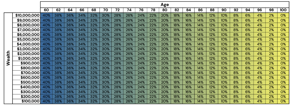
One solution to asset allocation through life is the typical “100 – age” method, where you are to subtract your age from 100, to obtain the percentage of equities to hold in your retirement portfolio. In theory, this heuristic is meant to reduce the impact of significant equity drawdowns as you near retirement, or death.
To tease the format of the figures to follow in this article, Figure 1 depicts how this typical equity allocation would appear in relation to both age, and wealth level. The allocation to bonds would encompass the remaining proportion of capital.
While many target-retirement products/strategies may provide a more sophisticated approach to retirement investing, the typical approach by many asset managers holds a high degree of similarity to this approach.
The other axis that this sort of heuristic ignores is life expectancy. It is entirely possible that an 80-year-old may be in better health than a 70-year-old, prompting the question of whether an investor or advisor may know that individual’s health situation better than a standardized table.
A logical question to then ask is: “If I have more-than-enough to live through retirement, should I be taking on more risk than necessary?” Conversely, “if I don’t have enough capital to make it through the next five years, how should I invest?”
This article seeks to answer that thread of questions.
Register for our Advisor Center
Tools Center:
Easily backtest & explore different return stacking concepts
Model Portfolios:
Return stacked allocations, commentary and guidance designed
for a range of client risk profiles and goals
Future Thinking:
Receive up-to-date insights into the world of return stacking theory and practice
Backwards Induction, or "Let's Assume We Had Enough at the End"
The “perfect” method to create a glidepath may not exist. It will also vary depending on many factors such as the goals of the investor, taxes, age, wealth level, dependents, inheritance desires, and many others.
One method to potentially simplify this problem is to utilize backwards induction. Gordon Irlam initially proposed a methodology such as this in Portfolio Size Matters (Journal of Personal Finance, Vol 13, Issue 2) to optimize for an investor that only wants their portfolio to sustain them through retirement. In other words, success is defined solely as dying before your money runs out. While our analysis is inspired by Irlam’s work, the analysis in this piece does not exactly mirror his approach, and we institute our own assumptions and methodologies to extend the framework.
That process works as follows:
- Starting at the end of life, assume that the investor had precisely enough capital, giving them a 100% success rate.
- Move back in time one year and generate 250,000 real return simulations for each of the included asset classes.
- For each relative wealth level and each random asset allocation, generate all 250,000 possible future wealth levels, subtracting the real withdrawal amount.
- For each randomly generated asset allocation possibility, set the success rate to the average success rate across all simulations. If a simulated asset allocation carries a 100% success rate, set the allocation equal to a 100% cash portfolio.
- For the given real spending unit level and years-until-retirement, find the top decile of the most successful asset allocations, and find the probability-weighted average success rate to set the portfolio configuration.
- Return to step 2.
Note that in this simplified example, there is no consideration of taxes, variability in spending patterns, or other sources of income (e.g. pension or social security).
Before we show the results, we would like to first note that instead of “wealth level” we are using “real spending units” (RSUs). It is easiest to define the term through an example. Assume we are planning on spending $50,000 per year, adjusted for inflation, and our retirement portfolio is worth $1,000,000. In such a case, RSUs would be equal to 20 ($1M / $50K). This is interpreted as the investor having 20 years of real spending power before the portfolio would run out of capital (assuming the portfolio were entirely invested in an asset that could match the rate of inflation).
Secondly, instead of age, we will be using “years until death”. While somewhat morbid, by presenting the data in this way, this allows the results to be generalizable, so they can be catered to an individual investor’s circumstances.
To begin, let us start with a straightforward stock/bond/cash allocation space.
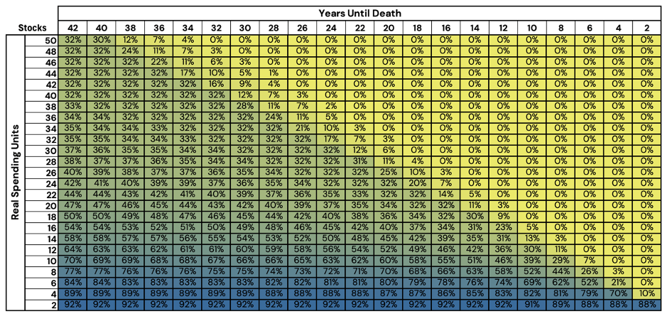
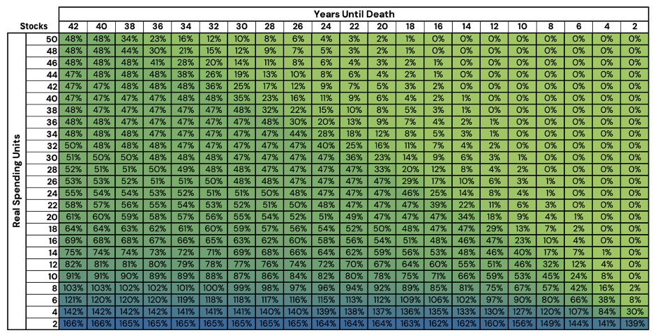
Figure 2: Optimized Stock/Bond/Cash Glidepath Allocations - Stocks
Source: Newfound Research, Bloomberg. For illustrative purposes, only. This should not be utilized as investment advice. You should consult a financial advisor before engaging in any investment activity. Stocks are represented by the FTSE All World Index (FTAW01 Index), Bonds are represented by the Bloomberg US Agg Total Return Value Unhedged USD Index (LBUSTRUU Index), and Cash is represented by the Bloomberg Short Treasury Total Return Index Value Unhedged (LD12TRUU Index).
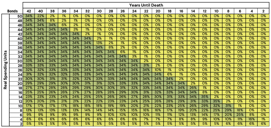
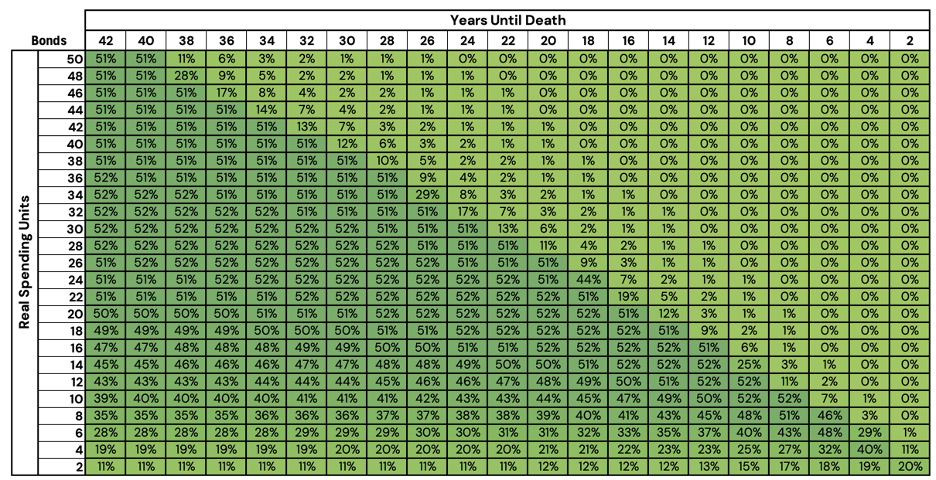
Figure 3: Optimized Stock/Bond/Cash Glidepath Allocation - Bonds
Source: Newfound Research, Bloomberg. For illustrative purposes, only. This should not be utilized as investment advice. You should consult a financial advisor before engaging in any investment activity. Stocks are represented by the FTSE All World Index (FTAW01 Index), Bonds are represented by the Bloomberg US Agg Total Return Value Unhedged USD Index (LBUSTRUU Index), and Cash is represented by the Bloomberg Short Treasury Total Return Index Value Unhedged (LD12TRUU Index).
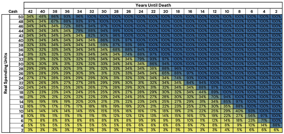
Figure 4: Optimized Stock/Bond/Cash Glidepath Allocation - Cash
Source: Newfound Research, Bloomberg. For illustrative purposes, only. This should not be utilized as investment advice. You should consult a financial advisor before engaging in any investment activity. Stocks are represented by the FTSE All World Index (FTAW01 Index), Bonds are represented by the Bloomberg US Agg Total Return Value Unhedged USD Index (LBUSTRUU Index), and Cash is represented by the Bloomberg Short Treasury Total Return Index Value Unhedged (LD12TRUU Index).
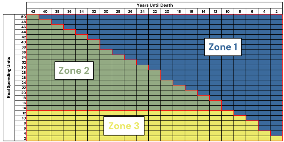
If we review the above figures, we can identify roughly three different zones that we can focus on for ease of understanding. Figure 4 shows a diagram of these zones for convenience.
Figure 5: Diagram of Glide Path Zones
Source: Newfound Research, Bloomberg. For illustrative purposes, only. This should not be utilized as investment advice. You should consult a financial advisor before engaging in any investment activity.
First, in the top-right corner of the graph, we see a large triangular region that is entirely dominated by a cash allocation. We may deem this region the “safe” region, or Zone 1. In this zone, an investor has a sufficient amount of wealth to fund their scheduled retirement spending. Despite a zero-to-negative real return on cash, the investor need not take any fixed income or equity risk to last through retirement.
In the middle-left, we see a zone (Zone 2) that is roughly equal weight between the three asset classes (from roughly 50 RSUs to 15). We can interpret this as the investor having too little capital for only cash to suffice, but a level of wealth most asset allocations hold a roughly equal probability of succeeding through retirement. A mixture of equities and bonds for real growth with cash cushioning against negative volatility.
It is important here to recall that we are defining success simply as dying before we run out of money. This creates an asymmetric goal for the optimization process, as we don’t care whether we die with $1 or $1,000,000. The optimizer is therefore likely to incorporate more cash than we might otherwise expect, as any excess volatility may reduce the portfolio’s chances of success.
Finally, in the bottom-left to bottom-right, we find a zone (Zone 3) where the equity allocations begin to grow substantially, as our wealth level decreases. This zone has an easy intuition behind it: if your capital is unlikely to last your full retirement, the investor needs to take on an increased degree of equity risk, in the hope of growing the portfolio into success.
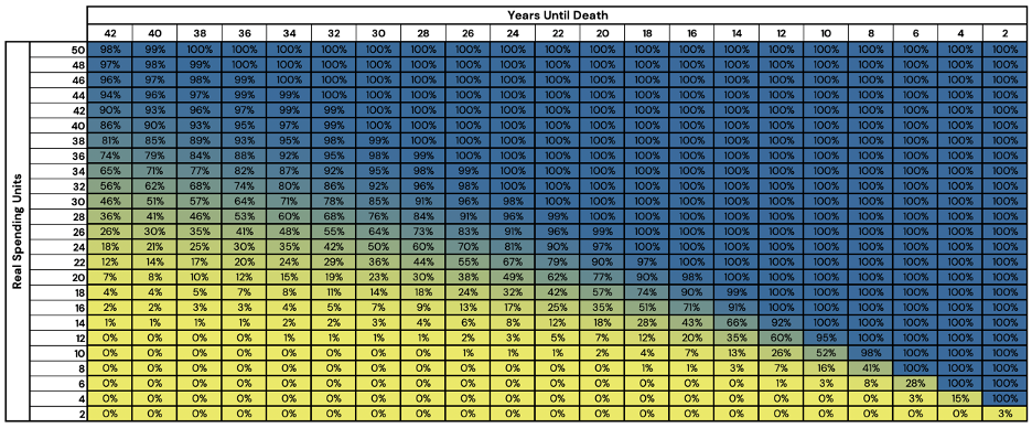
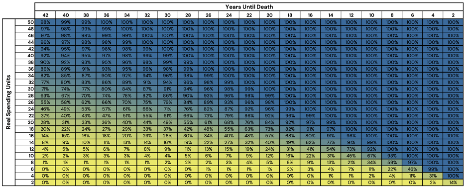
The simulated probability of success at each point of the glidepath can be found in Figure 6.
Figure 6: Probability of Success of Optimized Stock/Bond/Cash Portfolios
Source: Newfound Research, Bloomberg. For illustrative purposes, only. This should not be utilized as investment advice. You should consult a financial advisor before engaging in any investment activity. Stocks are represented by the FTSE All World Index (FTAW01 Index), Bonds are represented by the Bloomberg US Agg Total Return Value Unhedged USD Index (LBUSTRUU Index), and Cash is represented by the Bloomberg Short Treasury Total Return Index Value Unhedged (LD12TRUU Index).
One thing that immediately stands out to us, is the degree to which probability of success decreases, especially in early years of retirement. For example, with 42 years to the end of retirement, 30 RSUs holds a 10% advantage over 28 RSUs. The rapidity only increases as we near the end of our retirement, for example, 10 RSUs at 10 years to retirement has a 52% probability of success while 8 RSUs holds a 16% probability of success (a 36% decrease).
The Return Stacking landscape is ever evolving, go deeper by connecting with a team member.
How Can Return Stacking Help?
For investors that find themselves in Zone 1, where cash is entirely sufficient to cover spending needs, we are hard-pressed to find any reason for an investor to take on leverage. Levering cash is effectively equivalent to running in place, and adding any asset exposure in this zone creates downside risk (again, with no benefit given to the size of a bequeathment, volatility risk in this zone has zero marginal benefit).
Return stacking begins to become more interesting in Zone 2, and especially in Zone 3. In Zone 2, we can postulate that the ability to increase diversification and expected returns should increase success rates. In Zone 3, however, the optimal portfolio likely begins to take on additional risk, in the hopes of keeping up with the annual withdrawal rates.
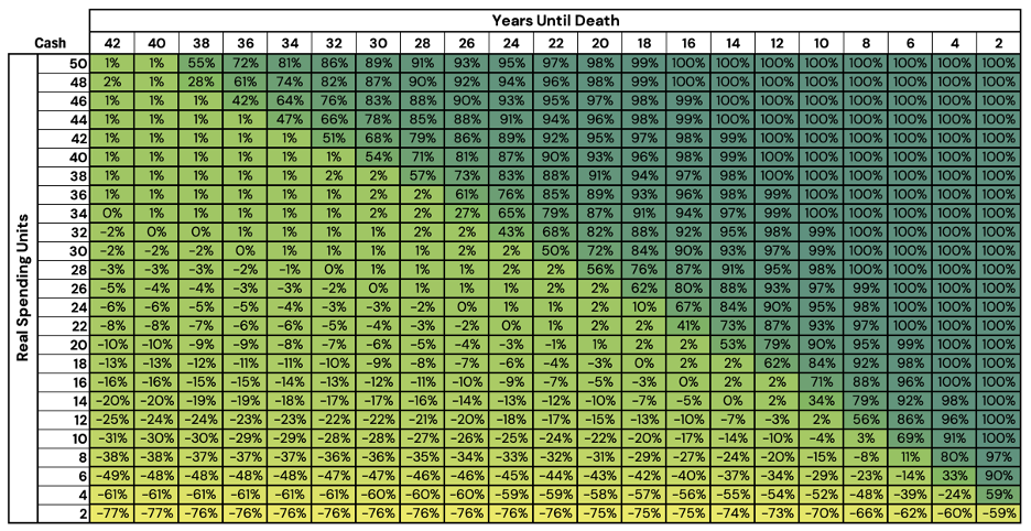
Figures 7, 8, and 9 show the equity, bond, and cash allocations when we allow the optimization program to take additional leverage up to a 200% notional allocation. Since we are allowing the preceding portfolios to take on leverage, for ease of interpretation, blue represents 200%, green represents roughly 50%, and yellow represents -100%.
Figure 7: Optimized Stock/Bond/Cash Glidepath Levered Allocations - Stocks
Source: Newfound Research, Bloomberg. For illustrative purposes, only. This should not be utilized as investment advice. You should consult a financial advisor before engaging in any investment activity. Stocks are represented by the FTSE All World Index (FTAW01 Index), Bonds are represented by the Bloomberg US Agg Total Return Value Unhedged USD Index (LBUSTRUU Index), and Cash is represented by the Bloomberg Short Treasury Total Return Index Value Unhedged (LD12TRUU Index).
Figure 8: Optimized Stock/Bond/Cash Glidepath Levered Allocations - Bonds
Source: Newfound Research, Bloomberg. For illustrative purposes, only. This should not be utilized as investment advice. You should consult a financial advisor before engaging in any investment activity. Stocks are represented by the FTSE All World Index (FTAW01 Index), Bonds are represented by the Bloomberg US Agg Total Return Value Unhedged USD Index (LBUSTRUU Index), and Cash is represented by the Bloomberg Short Treasury Total Return Index Value Unhedged (LD12TRUU Index).
Figure 9: Optimized Stock/Bond/Cash Glidepath Levered Allocations - Cash
Source: Newfound Research, Bloomberg. For illustrative purposes, only. This should not be utilized as investment advice. You should consult a financial advisor before engaging in any investment activity. Stocks are represented by the FTSE All World Index (FTAW01 Index), Bonds are represented by the Bloomberg US Agg Total Return Value Unhedged USD Index (LBUSTRUU Index), and Cash is represented by the Bloomberg Short Treasury Total Return Index Value Unhedged (LD12TRUU Index).
Before we discuss the results, we would like to point out that the cash allocations in Figure 9 have negative allocations. To clarify what this means, consider that if a portfolio holds a 125% notional allocation to risk assets, the portfolio will have to borrow the capital to obtain that additional 25% exposure: the portfolio will hold a -25% cash allocation. When figure 8 has a positive allocation, we can say that the portfolio is not taking any leverage, while when the cash allocation is negative, the optimizer is suggesting that taking on leverage is a prudent choice.
The results in figures 6, 7, and 8 align with our initial suspicions. In Zone 1, the cash allocation held a majority position, while in Zone 2, both stock and bond allocations increased, raising the expected return and diversification of the portfolio.
Finally, in Zone 3, we see that the equity allocation began quickly ramping up, while also maintaining a minor allocation to bonds, achieving a max notional exposure of 177%.
While the results match our intuition, how does the additional leverage impact our success rates?
Figure 10: Probability of Success of Optimized Levered Stock/Bond/Cash Portfolios
Source: Newfound Research, Bloomberg. For illustrative purposes, only. This should not be utilized as investment advice. You should consult a financial advisor before engaging in any investment activity. Stocks are represented by the FTSE All World Index (FTAW01 Index), Bonds are represented by the Bloomberg US Agg Total Return Value Unhedged USD Index (LBUSTRUU Index), and Cash is represented by the Bloomberg Short Treasury Total Return Index Value Unhedged (LD12TRUU Index).
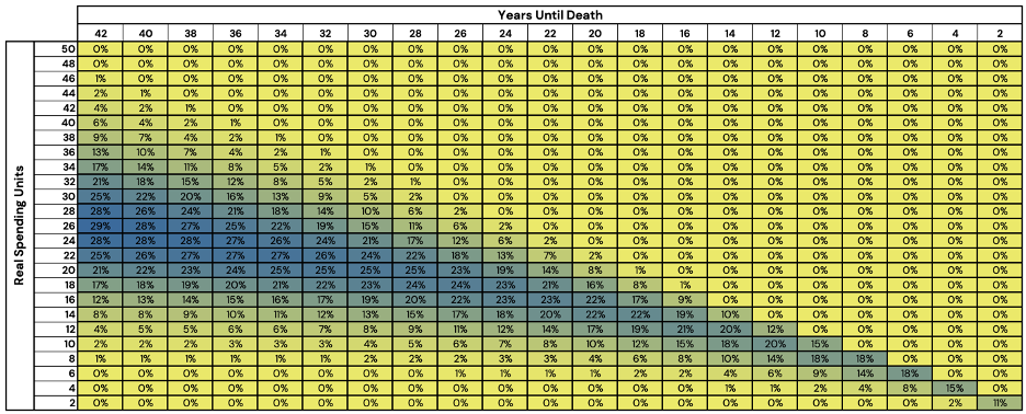
Figure 11: Success Rate Improvement Through Return Stacking
Source: Newfound Research, Bloomberg. For illustrative purposes, only. This should not be utilized as investment advice. You should consult a financial advisor before engaging in any investment activity. Stocks are represented by the FTSE All World Index (FTAW01 Index), Bonds are represented by the Bloomberg US Agg Total Return Value Unhedged USD Index (LBUSTRUU Index), and Cash is represented by the Bloomberg Short Treasury Total Return Index Value Unhedged (LD12TRUU Index).
The success rates in Zone 1, as expected, remains extraordinarily high at around 100% success. Zone 3 sees a relatively small increase in success rates, simply because it is almost impossible to outpace spending levels for more than a few years at that level of relative wealth.
Zone 2, does however, gets more interesting as we see a materially positive shift in success rates.
Additionally, an investor with 20 RSUs and 42 years left in retirement saw an increase of 16%. To convert this to more relatable numbers, an investor with a $1M portfolio taking an inflation-adjusted $50,000 withdrawal each year could increase her chances of success to 1-in-4 from 1-in-10 by incorporating return stacking into the portfolio.
Conclusion
In this article, we sought to provide an additional method of thinking about retirement investing which considers both the level of wealth and expected years in retirement. The analysis in this article specifically sought to find potentially optimal solutions when the investor’s goal is strictly to have enough capital to make it through retirement. While this may not be the only goal an investor may have, it provides a starting point and a reasonable goal that most investors aim to achieve.
Additionally, we sought to answer the question of whether the utilization of prudent leverage could increase our odds of success given this investment goal.
We found that the investment recommendations during retirement can be more personalized, beyond that of the “100 – Age” rule for allocations. The unlevered version of this analysis highlights the variations in allocation as we adjust both the relative wealth level and years until death. When there is not enough capital saved to ensure 100% success, utilizing return stacking can increase the chances that an investor’s capital will survive retirement.
In part 2 of this series on glidepath investing, we will increase the asset allocation space by including an additional diversifying asset, allowing us to compare how diversification, combined with return stacking, can impact success in retirement.
